The Short Version
This project is about choosing the best website variant for each visitor, using historical randomized logs. The winning approach is a support-aware hybrid: a leak-free empirical-Bayes table when data is thin, switching to a gradient-boosted T-learner once a segment has enough support to justify a more flexible functional form.
hybrid_eb_gbm average
hybrid_eb_gbm
as the workhorse policy. It uses the empirical-Bayes table when support
is thin, then switches to a gradient-boosted T-learner when enough data
exists. This keeps the sparse-data protection from seg_eb
while capturing nonlinear lift from gbm_tlearner.
Deliverables
The end deliverable is a public GitHub repo plus a recorded video. This HTML page is designed to be the "open this first" artifact for reviewers.
Code and repo
GitHub repository: https://github.com/jonathangu/coframe-personalization
solution/contains the submitted policies, write-up, generated results, and plots.solution/eb_policy.pycontains the final empirical-Bayes policy.solution/__init__.pyregisters every policy variant to preserve the research path.solution/report.htmlis this static report;solution/index.htmlforwards here.
Video
- Run the harness and show the score plots.
- Explain the contextual bandit framing and randomization.
- Walk through data displays and edge cases.
- Explain productionization: OPE, exploration, drift, and monitoring.
solution/report.html
locally in a browser, or push the repo and serve it with GitHub Pages.
All images use relative paths under solution/results/, so
the report stays portable when the repo moves online.
What We Are Solving
This is a one-step contextual bandit problem, not a full reinforcement learning problem. At a single moment, we observe context, choose one action, and get one reward.
Context
Visitor/session features: country, language, device, platform, referrer, returning status, visits, and timestamp.
Action
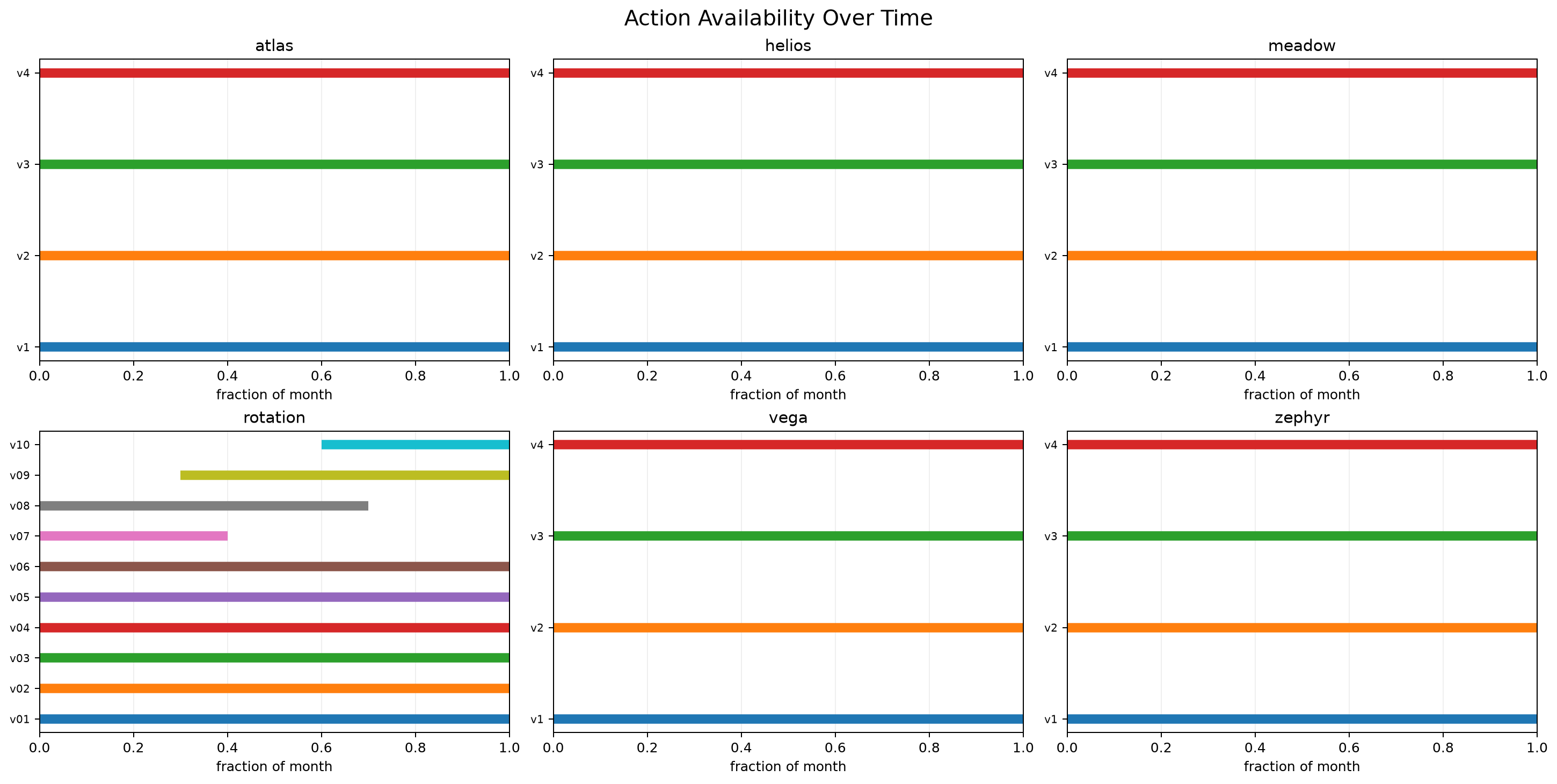
Choose one currently available variant_id. The action set can change, especially in rotation.
Reward
Binary conversion. In the log we only observe the reward for the variant that was actually shown.
For each visitor:
  x = context
  A = available variants
  choose a in A
  observe reward only for chosen a

Goal:
  estimate mu(x, a) = P(convert | context x, variant a)
serve argmax_a mu_hat(x, a) among available variantsWhat The Data Looks Like
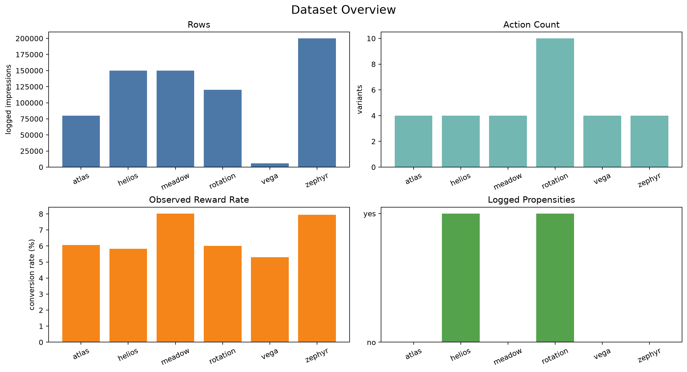
There are six datasets from May 2, 2025 through May 31, 2025. The observed logs are the only data the policy may train on. The hidden truth files are used by the evaluator and by offline diagnostics, not by the policy.
| Dataset | Rows | Variants | Observed reward | Feature feel | Special case |
|---|---|---|---|---|---|
| atlas | 80,000 | 4 | 6.07% | Standard visitor features | No headroom: all arms are effectively identical. |
| helios | 150,000 | 4 | 5.83% | Country/device/language signal | Non-uniform randomized assignment with propensities. |
| meadow | 150,000 | 4 | 8.02% | Country, language, platform, recency features | Clean contextual lift with uniform assignment. |
| rotation | 120,000 | 10 | 6.01% | Country and language dominate | Action set changes over time; propensities logged. |
| vega | 6,000 | 4 | 5.30% | Same schema but much less support | Sparse, high variance, easy to overfit. |
| zephyr | 200,000 | 4 | 7.94% | Country/referrer/language signal | Concept drift: recent data matters more. |
Randomization And Propensity Refresher
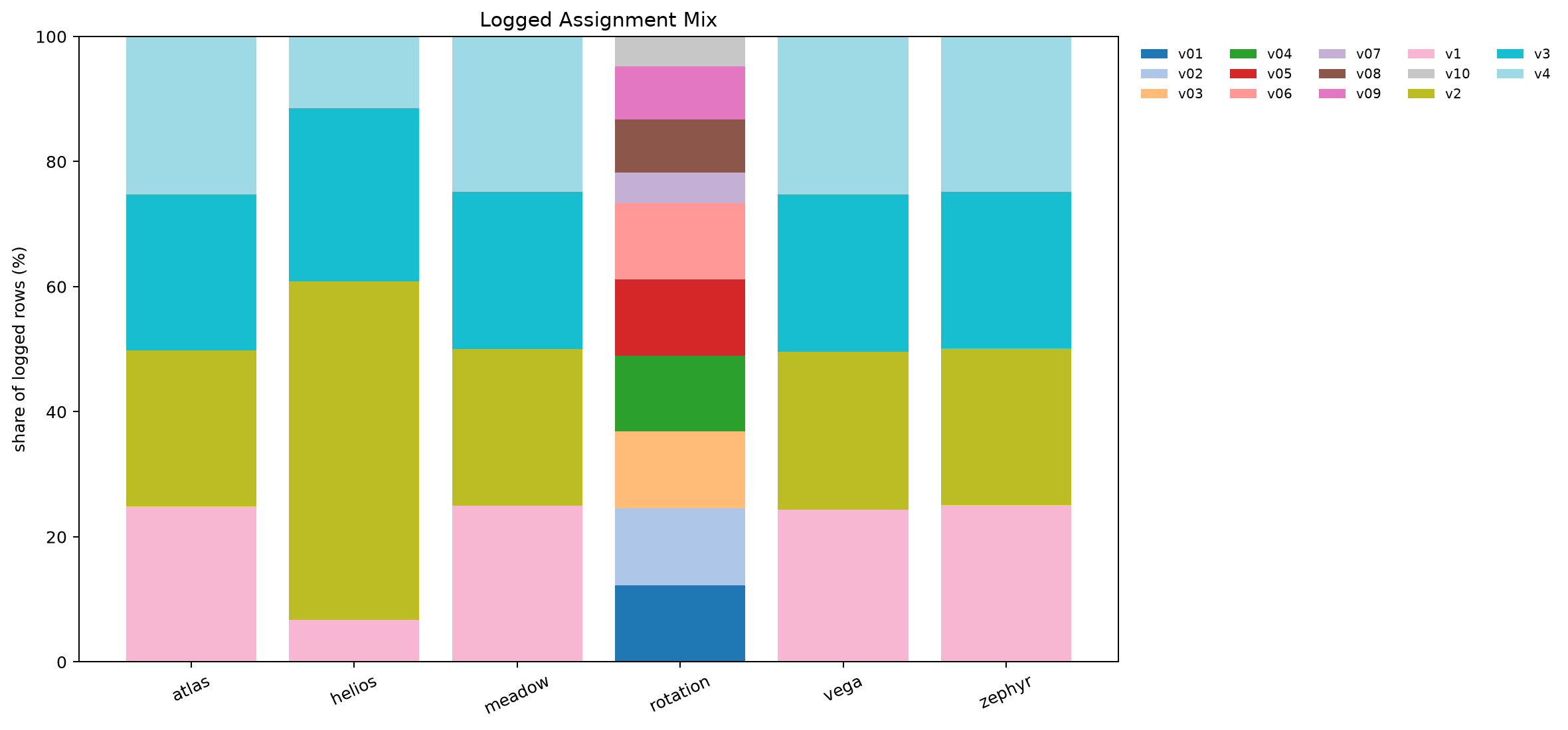
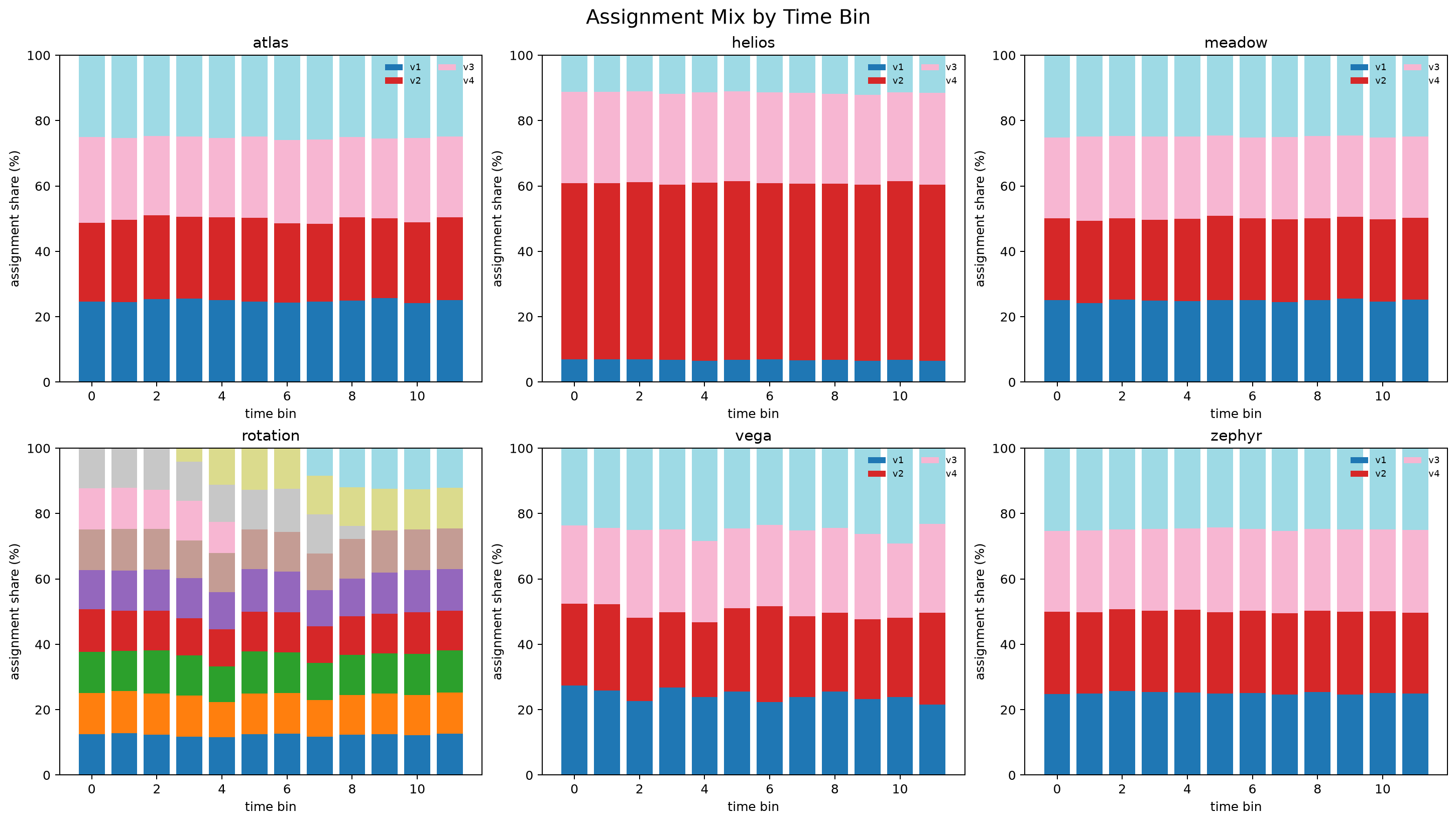
The logs are randomized, but not always uniformly randomized. That is the key distinction. Some datasets show each variant about equally often; others use a known logging probability called a propensity.
| Dataset | Assignment pattern | What to condition on | Policy implication |
|---|---|---|---|
| atlas, meadow, vega, zephyr | Near uniform random assignment, about 25% per arm. | Context is enough; implicit propensity is about 1/K. |
Use ordinary direct outcome modeling with shrinkage. |
| helios | Non-uniform randomized assignment: propensities include 0.05, 0.25, 0.85. | Assignment is random conditional on the logging propensity/context. | Use propensity as a diagnostic; raw IPW is high variance. |
| rotation | Random among live variants while variants enter and leave. | Condition on time/action availability; propensity is about 1/8 or 1/9. | Always mask recommendations to available_variants. |
Do we need to condition on "the chance this person was assigned"?
Conceptually, yes: causal comparisons need the assignment mechanism.
Practically, the final policy estimates E[reward | context, action]
using the randomized log and heavy shrinkage. For uniform datasets,
the propensity is just a constant. For helios, a logged
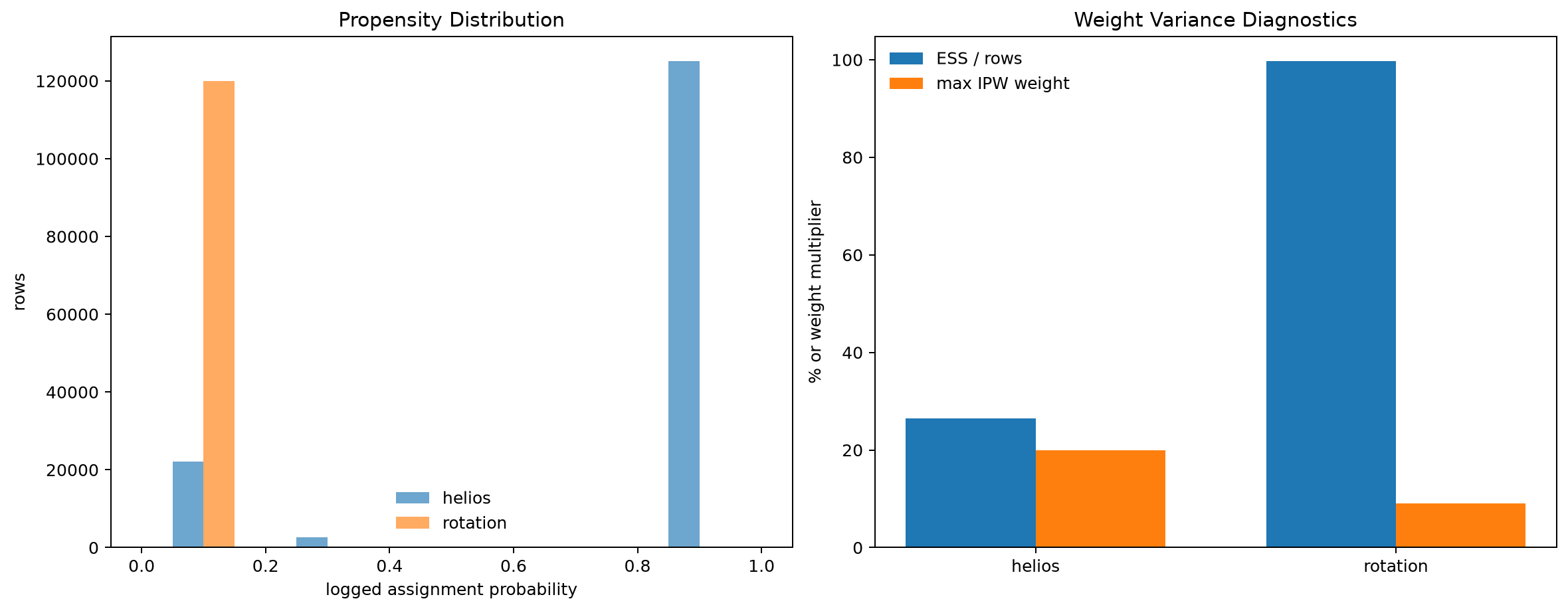
propensity of 0.05 means a raw 1 / propensity weight of 20,
so a few rows can dominate and inflate variance — the safer scored policy
is direct outcome modeling with support-aware shrinkage. In production OPE, propensities become
central again because we will not have hidden truth files.
Variance, Small Weights, And Shrinkage
The user insight that matters most is variance: when propensities are small, inverse-propensity weights are huge. A technically unbiased estimate can still be useless for choosing an action if it is too noisy.
Inverse propensity weight:
  weight_i = 1 / P(action_i was assigned | context_i)

Example:
  propensity = 0.05
  weight = 20

Effective sample size:
  ESS = (sum weights)^2 / sum(weights^2)
The risk
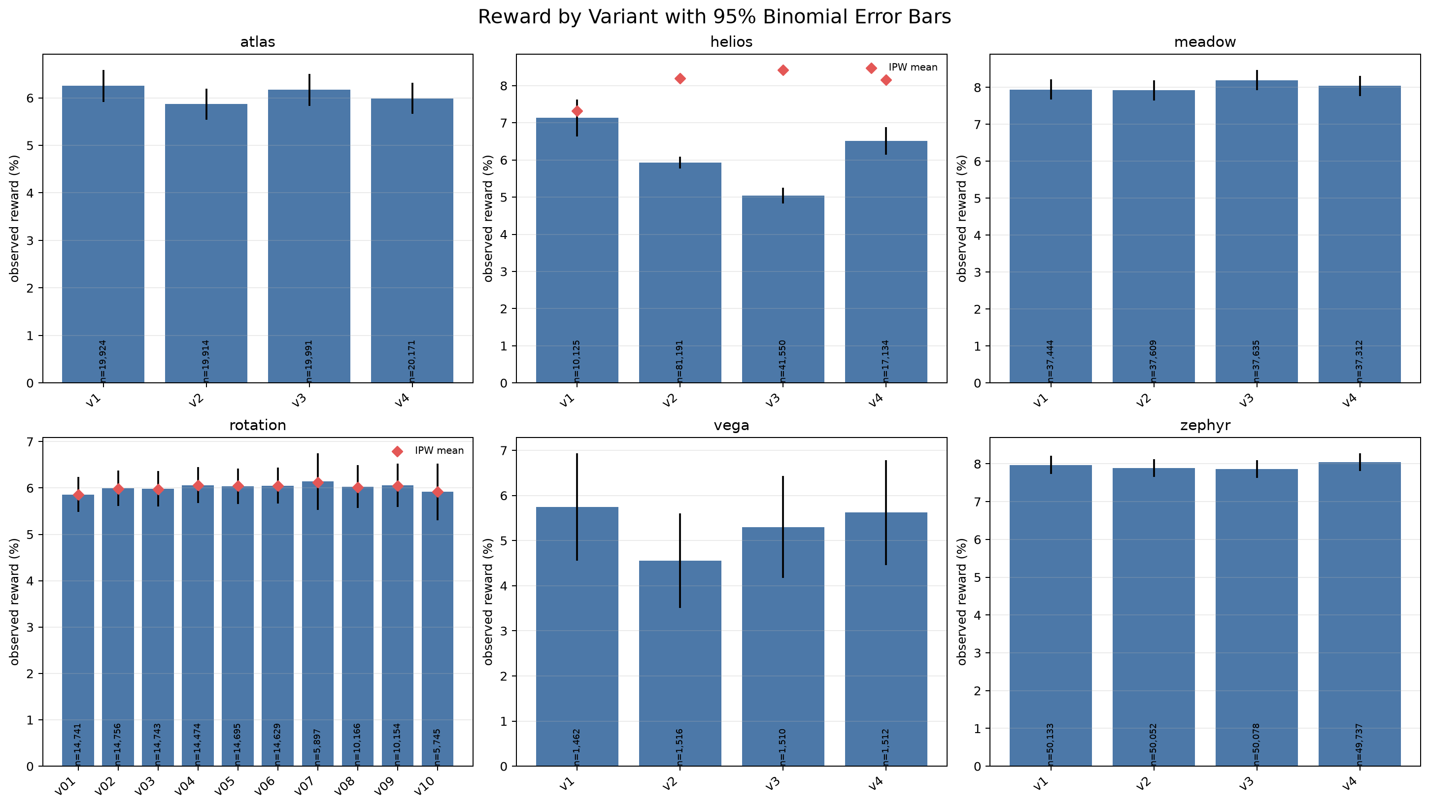
A single lucky conversion in a rare cell can make a variant look
amazing. If the policy greedily picks the noisy winner, it overfits.
This is especially dangerous in helios and vega.
The fix
Empirical-Bayes shrinkage: estimate every segment/variant cell, but pull thin cells back toward a stable parent rate. As support grows, the data earns the right to move the score.
The Harness
The evaluator mimics production by walking forward in time. Training always happens before the window being scored.
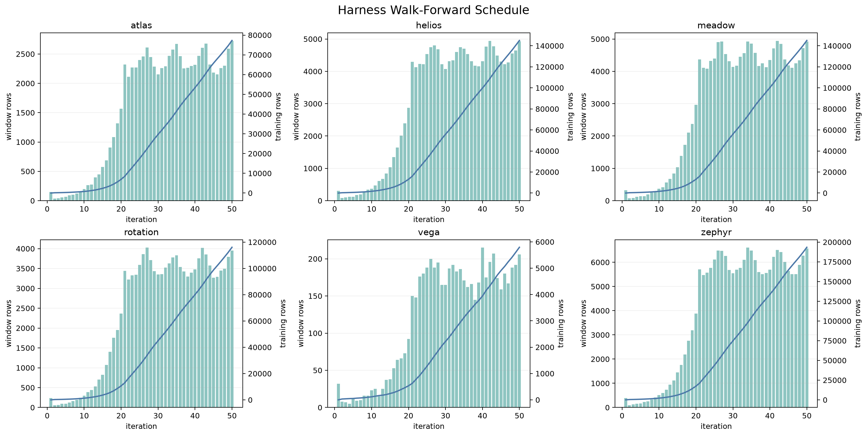
score_variants() must
return columns in meta.variant_ids order, not
available_variants order. The EB policy explicitly follows
this contract, then the base ScoredPolicy masks unavailable
arms safely.
Implementation
The final policy is a support-adaptive direct reward model. It starts with an additive empirical-Bayes T-learner, then switches to a histogram-gradient-boosted T-learner once the training history is large enough for flexible nonlinear modeling.
Registered policies
random my_policy best_fixed example feature_demo seg_country seg_eb seg_eb_recency gbm_tlearner hybrid_eb_gbm lgbm_tlearner hybrid_eb_lgbm
Final files
solution/eb_policy.py implements the conservative EB
component. solution/gbm_policy.py implements the GBM
T-learner and final hybrid. The observability scripts generate the
data, harness, and arm-sensitivity displays used in this report.
EB policy formula
score(context x, variant a)
  = logit(global_arm_prior[a])
    + sum_feature deviation(feature_value, a)
    + sum_cross deviation(cross_value, a)

shrunk_rate(segment, a)
  = (reward_sum(segment, a) + k * parent_prior[a])
    / (count(segment, a) + k)
GBM and hybrid logic
gbm_tlearner:
  for each arm a:
    fit HistGradientBoostingClassifier on rows where variant_id == a
    predict P(reward=1 | x, arm=a)

hybrid_eb_gbm:
  if n_train < 50,000 or any arm has fewer than 2,000 rows:
    use seg_eb
  else:
    use gbm_tlearner
What it uses
- Categorical features from the harness metadata.
- Numeric features binned on training data only.
- Country crossed with language, device type, and platform.
- Optional recency weighting for drift experiments.
- Gradient-boosted trees when support is large enough.
What it avoids
- No truth-file access during policy training.
- No target encodings fit on the scored window.
- No raw propensity as a serving feature.
- No noisy personalization when a cell lacks support.
- No dataset-name hard-coding in the hybrid switch.
What Kind Of ML Model Is This?
The shipped model is a direct-method, multi-action T-learner for a contextual bandit. The final submitted policy is a hybrid: EB shrinkage for low-support regimes, gradient boosting for high-support regimes. Both estimate the expected conversion rate for every variant in the current context, then choose the highest score among live variants.
The exact model shape
hybrid_eb_gbm is a support-gated T-learner. "T-learner"
means each action has its own estimated outcome surface:
mu_a(x) = E[reward | context = x, action = a]

serve:
  choose argmax_a mu_hat_a(x)
  subject to a being in available_variants
In low-support windows, the policy uses shrunk segment tables in log-odds space. The prediction for a variant is:
score(x, a)
  = global arm prior
    + country effect for arm a
    + language effect for arm a
    + platform/device/numeric-bin effects for arm a
+ selected country-cross effects for arm aIs this uplift modeling?
It is related, but the final policy is not only an "uplift model" in the narrow binary-treatment sense. Classic uplift modeling asks, "How much better is treatment than control for this user?" Here there are multiple variants and every visitor must receive one of them. We can express the decision as uplift against a baseline:
uplift_a(x) = mu_a(x) - mu_baseline(x)
But because the baseline term is common when comparing arms, choosing the
largest mu_a(x) gives the same action as choosing the largest
uplift. So the submitted policy models absolute reward per action, while
the business interpretation is "personalized lift over best fixed."
How T, X, and R learners fit
| Approach | What it learns | Fit for this take-home |
|---|---|---|
| T-learner | One outcome model per action: mu_a(x). |
Chosen. EB and GBM are both T-learners in this submission. |
| S-learner | One model with action included as a feature. | Possible, but can underfit action-by-context flips unless interactions are learned well. |
| X-learner | Imputes treatment effects, usually for binary treatment/control. | Useful with imbalanced treatment/control data, but awkward for many variants and unnecessary here. |
| R-learner | Residualized heterogeneous treatment effects after modeling outcome and propensity nuisances. | Strong for observational causal inference; more machinery than needed for randomized logs and hidden-truth scoring. |
| Doubly robust learner | Outcome model plus propensity-corrected residuals. | Excellent production/OPE idea. In this scored benchmark, raw propensity correction can add variance. |
| GBM/LightGBM T-learner | Flexible per-arm tree models. | Implemented as gbm_tlearner. Strong on large/drifting datasets, weak on sparse vega. |
| Support-adaptive hybrid | Use EB until there is enough data, then switch to GBM. | Final policy. Best average score: 69.6% captured headroom. |
| Bandit exploration algorithms | UCB, Thompson sampling, epsilon-greedy logging policies. | Production exploration, not the offline score. The benchmark rewards best current exploitation. |
Walk-forward retraining, not RL
We are not discovering by changing the future data collection process in this benchmark. The harness replays fixed historical windows. At each time step, we train only on the past and score on the next unseen window:
iteration 11:
  train on all data through iteration 10
  recommend for iteration 11

iteration 15:
  train on all data through iteration 14
  recommend for iteration 15
That is why there is no data leakage: the model can keep retraining as time moves forward, but it never uses reward, action, or truth from the window it is currently scoring.
How to think about stale data and drift
Stale data matters when P(reward | context, action) changes over
time — then old rows are not just less fresh, they are actively
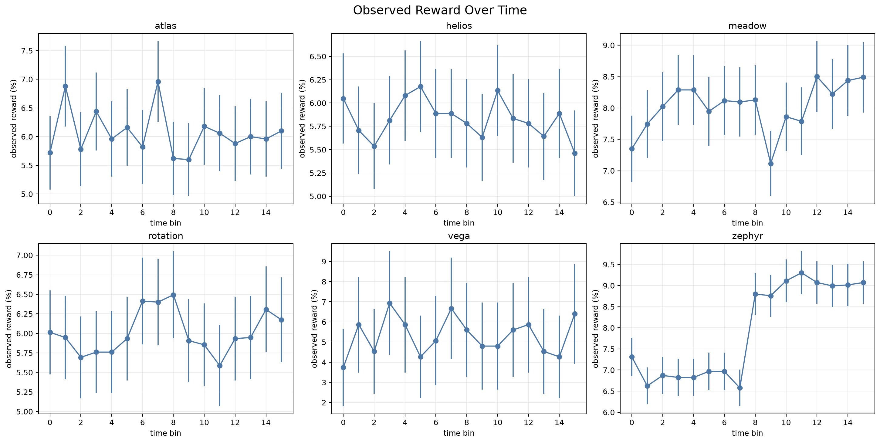
misleading. zephyr is the case: the best arm flips
at the midpoint of the timeline.
| zephyr — true CVR | variant_2 | variant_1 |
|---|---|---|
| first half | 12.06% | 2.69% |
| second half | 3.94% | 13.31% |
A full-history model averages two incompatible regimes, so it keeps "remembering"
that variant_2 used to be great and adapts too slowly. Recency
weighting discounts old rows — weight = 0.5 ** (age_days / half_life),
so with a 4-day half-life a row 8 days old counts as a quarter of a row. That is
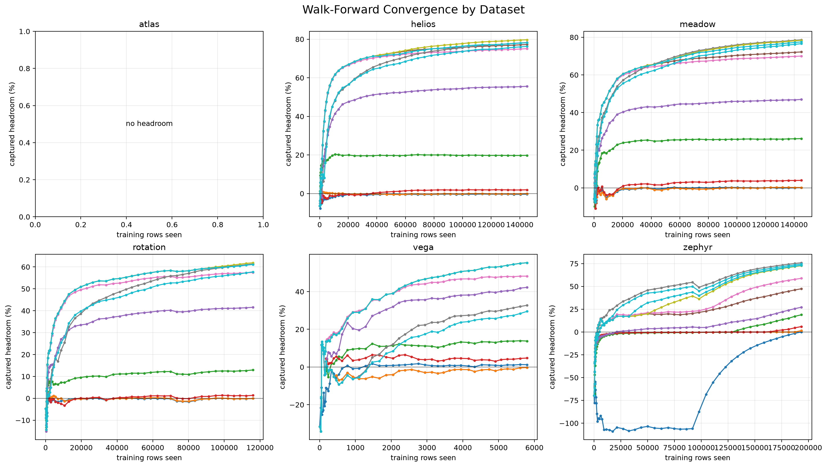
why on zephyr: EB full-history 47.4% → EB recency
58.9%, and the time-aware gbm_tlearner reaches
75.9%.
But recency is not free: it trades bias from stale data for variance from a smaller effective sample size. Forgetting old rows on a stable dataset throws away valid signal. A single global 4-day half-life proved this — it helped zephyr but hurt every stationary dataset:
seg_eb_recency − seg_eb | zephyr | helios | meadow | rotation | vega |
|---|---|---|---|---|---|
| Δ captured headroom (pts) | +11.5 | −2.2 | −2.2 | −3.7 | −7.1 |
vega is hit hardest (−7.1) because it already has only 6,000 rows —
recency made a sparse problem sparser. So "always weight recent data higher" isn't
wrong, it's a bias-variance choice: keep long memory while
the process is stable, switch to short memory only once it has changed.
Current stale-data tool
seg_eb_recency applies exponential time decay. The
gbm_tlearner also includes timestamp-derived features,
letting trees split on recent regimes. These both prove the drift
hypothesis on zephyr.
Better production version
Use adaptive recency. Keep all history while the process is stable; turn on decay only when monitoring detects a change in reward rates, arm rankings, calibration, or segment-level residuals.
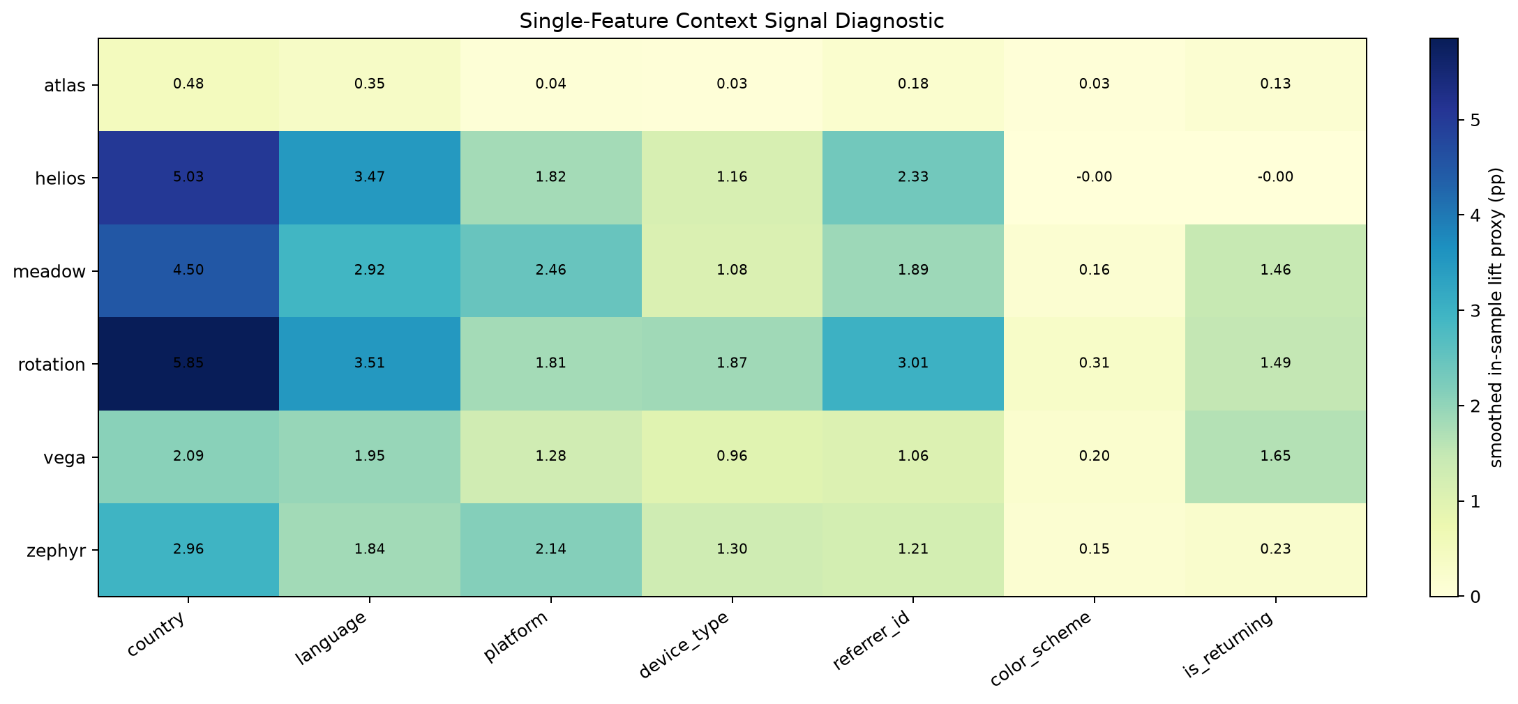
Observability Displays
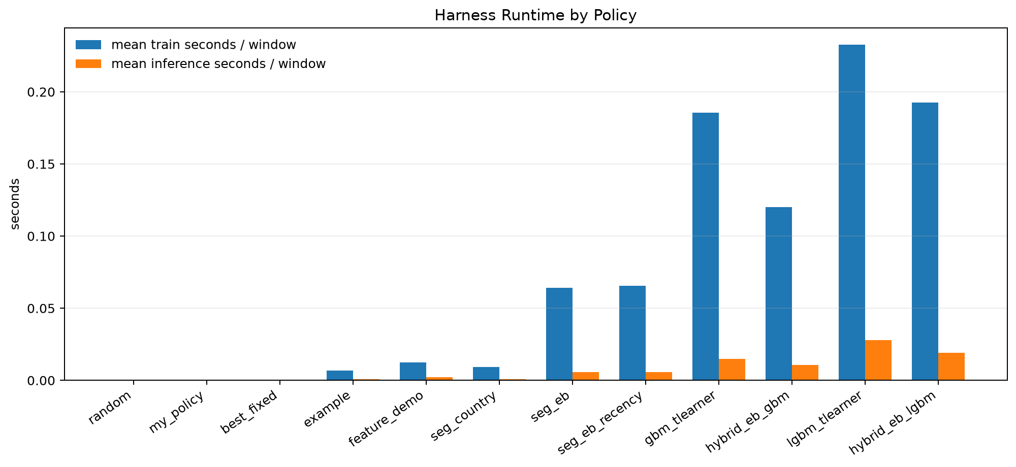
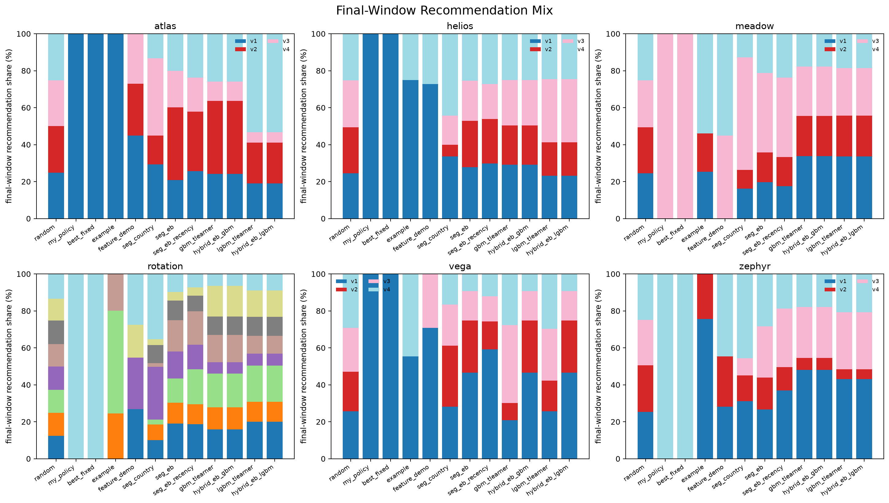
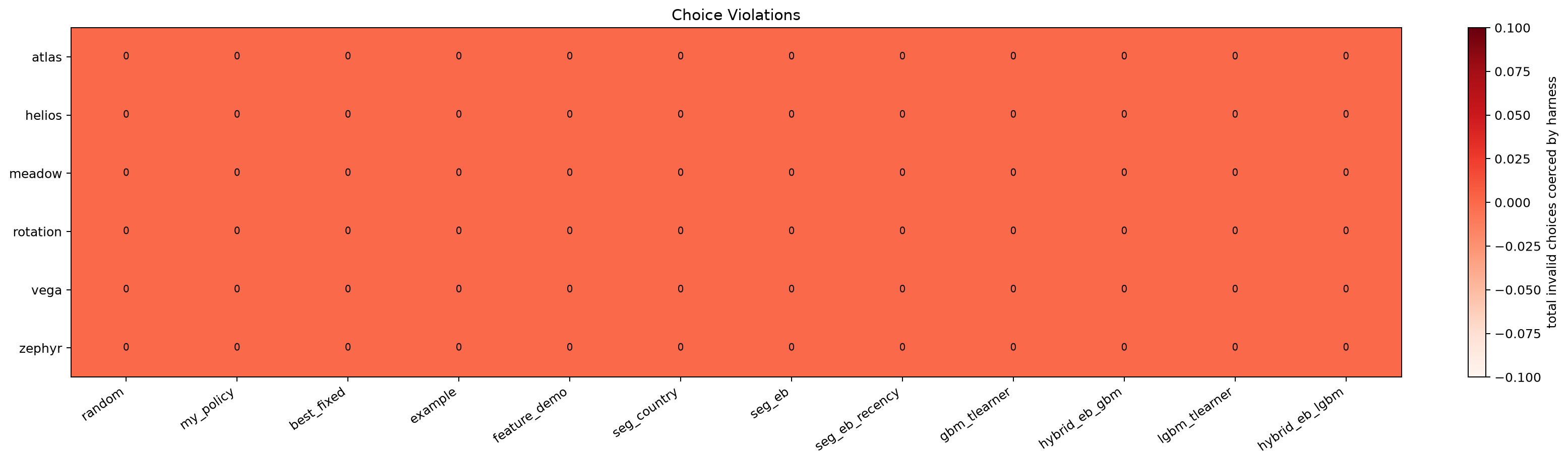
These plots make the data and harness inspectable. They are useful for the video because they show why the final policy is shaped the way it is.
Results
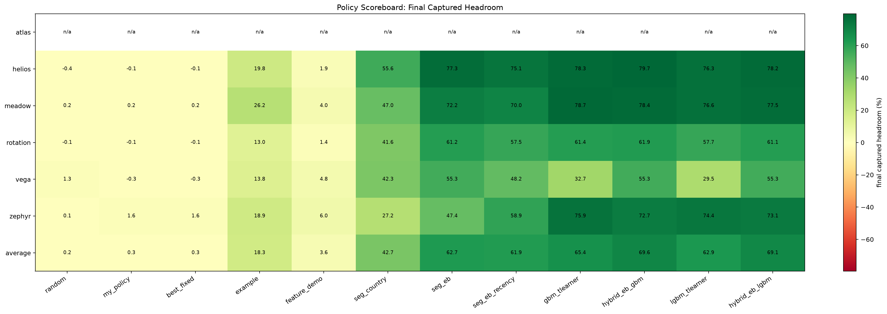
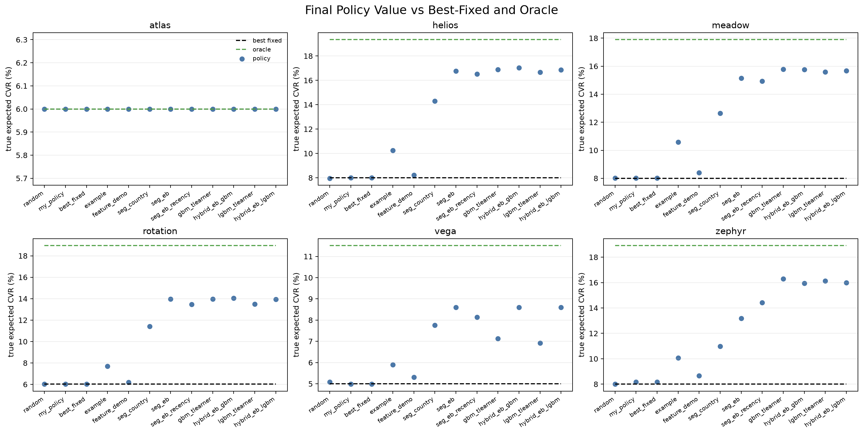
Full walk-forward evaluation over 50 iterations, comparing the starter baselines, provided examples, our data-display experiments, and the final EB policies.
| Policy | Atlas | Helios | Meadow | Rotation | Vega | Zephyr | Avg headroom datasets |
|---|---|---|---|---|---|---|---|
random |
n/a | -0.4% | 0.2% | -0.1% | 1.3% | 0.1% | 0.2% |
my_policy |
n/a | -0.1% | 0.2% | -0.1% | -0.3% | 1.6% | 0.3% |
best_fixed |
n/a | -0.1% | 0.2% | -0.1% | -0.3% | 1.6% | 0.3% |
example |
n/a | 19.8% | 26.2% | 13.0% | 13.8% | 18.9% | 18.3% |
feature_demo |
n/a | 1.9% | 4.0% | 1.4% | 4.8% | 6.0% | 3.6% |
seg_country |
n/a | 55.6% | 47.0% | 41.6% | 42.3% | 27.2% | 42.7% |
seg_eb |
n/a | 77.3% | 72.2% | 61.2% | 55.3% | 47.4% | 62.7% |
seg_eb_recency drift ablation |
n/a | 75.1% | 70.0% | 57.5% | 48.2% | 58.9% | 61.9% |
gbm_tlearner |
n/a | 78.3% | 78.7% | 61.4% | 32.7% | 75.9% | 65.4% |
hybrid_eb_gbm shipped |
n/a | 79.7% | 78.4% | 61.9% | 55.3% | 72.7% | 69.6% |
lgbm_tlearner |
n/a | 76.3% | 76.6% | 57.7% | 29.5% | 74.4% | 62.9% |
hybrid_eb_lgbm |
n/a | 78.2% | 77.5% | 61.1% | 55.3% | 73.1% | 69.1% |

Why the hybrid wins
hybrid_eb_gbm is not a new model — it is a per-window
router between two base learners with opposite error profiles, gated on
a leak-free signal: how much training data exists so far.
seg_eb — empirical-Bayes table
- Low variance. Shrinks thin cells to stable priors; never overreacts to a handful of rows.
- Some bias. Additive (mains + a few crosses) — cannot represent arbitrary interactions or time structure.
- Best when data is sparse or early.
gbm_tlearner — boosted trees
- Low bias. Captures arbitrary interactions and uses a time/age feature, so it tracks drift.
- High variance. Overfits thin cells — on sparse
vegait collapses to 32.7%. - Best when data is large and the signal is nonlinear or non-stationary.
The switch is on support, every window
each walk-forward window:
  if len(train) >= 50,000  AND  every arm has >= 2,000 rows:
      use gbm_tlearner        # rich enough to trust the flexible model
  else:
      use seg_eb              # sparse / early -> shrink, do no harm
The gate reads only training support, so it is leak-free. Because it runs every window, it is also a cold-start-to-mature switch over time: the data-poor early windows use EB (which converges faster from little data), and once history is large the same dataset graduates to GBM.
What the gate produces, dataset by dataset
| Dataset | seg_eb | gbm | hybrid | What the gate did |
|---|---|---|---|---|
vega · 6k rows | 55.3 | 32.7 | 55.3 | Never reaches 50k → always EB. Avoids GBM's 23-point collapse. |
zephyr · 200k, drift | 47.4 | 75.9 | 72.7 | Graduates to GBM, whose time feature tracks the regime flip. +25 over EB. |
meadow · 150k | 72.2 | 78.7 | 78.4 | GBM captures the interactions EB can't. +6 over EB. |
helios · 150k | 77.3 | 78.3 | 79.7 | Beats both — EB early, GBM late, summed over the walk-forward. |
rotation · 120k, 10 arms | 61.2 | 61.4 | 61.9 | 10 arms keep some windows under 2k/arm → conservative; edges both. |
atlas · no headroom | n/a | n/a | n/a | Nothing to learn; do no harm. |
vega — and because it
defaults to EB unless support is clearly large, it can never be much worse than the
safe baseline. It is a guarded ensemble — model selection on a leak-free
signal, the principled answer to "which functional form?": it depends
on support, so decide per window. This is exactly what the arm-sensitivity
analysis prescribed — GBM's disagreements with EB add value where data is
rich and destroy it where it is thin.
Edge Cases
These are the cases to call out in the video. They show that the solution is not just chasing a leaderboard number.
| Dataset | What is tricky | How the policy handles it |
|---|---|---|
| atlas | No personalization headroom; oracle equals best fixed. | Shrinkage collapses noisy effects to priors; captured% is correctly n/a. |
| helios | Non-uniform assignment and tiny propensities. | Raw arm averages are biased, but reward modeling is valid conditional on context; avoid raw IPW (0.05 → weight 20). Hybrid reaches 79.7%. |
| rotation | Variants enter and leave over time. | Scores canonical arms, then masks to available variants; reaches 61.2%. |
| vega | Only 6,000 rows; sparse cells. | Heavy EB shrinkage avoids overreacting; reaches 55.3%. |
| zephyr | Concept drift. | Base EB captures 47.4%; recency version reaches 58.9% but hurts stationary datasets. |
Productionization
In production there is no truth file and no guaranteed clean randomization. The machinery we deliberately set aside for the offline score — propensities, off-policy evaluation, exploration, drift handling — is exactly what comes back.
Off-policy evaluation when counterfactuals are unavailable
Offline here we score against the hidden per-arm oracle. In production there is no oracle, so you estimate a new policy's value from logged data. The doubly-robust (DR) estimator is the workhorse — it combines a reward model with propensity weighting:
V_DR(pi) = average over logged rows of:
    m_hat(x, pi(x))                                # reward-model guess for the new policy's choice
  + 1{a == pi(x)} / p(a | x) * ( y - m_hat(x, a) ) # correction, ONLY when the log happened to show
                                                   # the same arm the new policy would have chosen
It is "doubly robust" because the estimate stays consistent if either the
reward model or the propensities are correct — two parachutes, you only
need one to open. Intuition: start from the model's prediction; on the rows where
the logged arm matches the new policy's choice, correct it by the
propensity-weighted residual (actual − predicted).
SNIPS (self-normalized) and weight clipping tame
the variance that small propensities create.
p(a|x) ≈ 0 and the correction term
explodes — no estimator recovers counterfactuals the data barely contains. That is
the same variance story as the helios ESS drop (150k → ~40k under raw
IPW), and it is why production keeps exploration alive and logs a propensity
for every served decision.
Exploration vs. greedy exploitation
Greedy argmax is optimal for this offline score, but in
production greedy starves the arms it disfavors — without
overlap you can no longer estimate those arms, and the model decays. You keep a
controlled amount of exploration (Thompson sampling or
ε-greedy, or a small randomized holdout) to preserve overlap and keep OPE valid.
This is the Fisher-information / value-of-information idea, scoped concretely:
spend exploration where an arm's value confidence interval still overlaps the
current argmax and the segment is high-traffic — i.e. where information
is both uncertain and decision-relevant.
Retraining cadence
Keyed to drift, not a fixed clock. Monitor per-arm and
per-segment CVR and the model's rolling log-loss; a change-point detector
(CUSUM / Bayesian online change-point) triggers down-weighting of stale data —
the adaptive version of seg_eb_recency. zephyr is the
cautionary tale: a static expanding-window model craters when the best arm flips
mid-stream, while an adaptive one recovers within a few windows.
Serving latency
The empirical-Bayes table is a hash lookup plus argmax — microseconds
per impression, trivially cacheable. A per-arm gradient-boosted model
costs n_arms model evaluations per impression (10× on
rotation's ten arms). The shipped hybrid_eb_gbm serves
the cheap EB path for thin segments and the GBM only where support justifies it,
so most traffic takes the fast path; hot-segment GBM scores can be precomputed
and cached if needed.
atlas.
Learnings And Discussion
This section consolidates the discussion from our thread, the local research log, and the parallel agent's strategy notes.
What we learned
- The target is simple: choose the arm with the highest expected conversion for this context.
- The hard part is estimation under missing counterfactuals, sparse cells, drift, and changing actions.
- Propensities matter for identification and OPE, but raw IPW can hurt the scored policy through variance.
- Shrinkage is the main protection against noisy argmax decisions.
- Recency is valuable only when drift exists; it should become adaptive.
What we implemented
- Data observability displays for assignment, reward, propensities, availability, and segment signal.
- Eval observability displays for scoreboard, convergence, runtime, recommendation mix, and violations.
- A country-only EB policy as an interpretable rung.
- A full additive EB policy with categorical/numeric features and selected crosses.
- A recency-weighted EB variant to test drift.
What came from the parallel work
The parallel strategy file emphasized the same core framing: this is a
contextual bandit, not RL; the scoring oracle makes greedy exploitation
appropriate for the take-home; propensities should be handled carefully;
and EB shrinkage is the right response to sparse or high-variance cells.
It also flagged two important harness details we adopted: the stored
oracle_value behavior on rotation, and the
canonical score_variants column-order contract.
What is next
- Adaptive recency: keep the zephyr gain without hurting stationary datasets.
- Propensity experiment: add clipped/stabilized IPW as a measured ablation, mainly for helios and rotation.
- LightGBM tuning: tune the LightGBM hybrid (currently ~69.1% on first-pass hyperparameters) to match or beat the sklearn hybrid, as the faster production backend.
- Production OPE: add IPS/SNIPS/doubly robust evaluation with confidence intervals.
- Exploration design: use Fisher-information or optimal-design thinking to collect data where uncertainty is decision-relevant.
Video Outline
This is the clean story for the recorded submission. The goal is to sound rigorous without burying the reviewer in implementation detail.
| Time | Segment | What to show |
|---|---|---|
| 0:00-0:30 | Framing | Open this report. Context, action, reward; why this is an offline contextual bandit, not RL. |
| 0:30-2:00 | 1 · Demo | Run uv run run_eval.py --policies random,my_policy,seg_eb,gbm_tlearner,hybrid_eb_gbm then uv run plot_results.py. Read the captured-headroom report as it prints; show each rung beat the last and the random baseline, on the scoreboard + convergence plots. |
| 2:00-4:00 | 2 · Solution & research log | Walk the research log: how I profiled the datasets (randomization, propensity, signal, drift), the policy ladder and what drove each step, and the arm-sensitivity analysis. Name every AI tool and test harness used (Claude Code + a parallel agent thread, the walk-forward eval harness, the observability scripts, scikit-learn then LightGBM). |
| 4:00-5:15 | 3 · Edge cases | atlas = no headroom (do no harm), vega = sparse/underpowered, zephyr = concept drift, rotation = changing action set, helios = non-uniform randomized logging, plus the cold start. Show which dataset exhibits each and how the policy holds up. |
| 5:15-6:45 | 4 · Productionization | OPE without counterfactuals (IPS / SNIPS / doubly-robust, and the ESS drop on helios), exploration vs. greedy exploitation, retraining cadence / drift detection, and serving latency. |
| 6:45-7:00 | Close | Recap: 69.6% average captured headroom for hybrid_eb_gbm; point to the repo and this hosted page. |
Runbook
Commands used to reproduce the policy comparisons and regenerate this report's figures.
uv run run_eval.py --policies random,my_policy,best_fixed,example,feature_demo,seg_country,seg_eb,seg_eb_recency,gbm_tlearner,hybrid_eb_gbm,lgbm_tlearner,hybrid_eb_lgbm --workers 1 --threads 2
uv run plot_results.py
uv run python solution/observability.py
uv run python solution/eval_observability.py
uv run python solution/arm_sensitivity.py
solution/eb_policy.py - final EB policy
solution/__init__.py - policy registration
solution/research_log.md - research log
solution/submission_checklist.md - submission checklist
solution/observability.py - data displays
solution/eval_observability.py - eval displays
solution/results/summary.json - full eval summary
solution/results/eval.log - printed eval log
Exact full-run summary
AVERAGE across headroom datasets (helios, meadow, rotation, vega, zephyr)
  random         mean captured=   0.2%
  my_policy      mean captured=   0.3%
  best_fixed     mean captured=   0.3%
  example        mean captured=  18.3%
  feature_demo   mean captured=   3.6%
  seg_country    mean captured=  42.7%
  seg_eb         mean captured=  62.7%
  seg_eb_recency mean captured=  61.9%   (drift ablation; helps zephyr, hurts stationary)
  gbm_tlearner   mean captured=  65.4%   (boosted trees; overfits sparse vega -> 32.7%)
  hybrid_eb_gbm  mean captured=  69.6%   <-- SHIPPED: EB when thin, GBM when rich
  lgbm_tlearner  mean captured=  62.9%   (LightGBM backend; faster than sklearn)
  hybrid_eb_lgbm mean captured=  69.1%   (LightGBM hybrid; ~same score, faster)